02
JanChristmas Offer : Get Flat 50% OFF on Live Classes + $999 Worth of Study Material FREE! - SCHEDULE CALL
Comparison of two population-related data refers to the practice of finding the difference between two different population-related data created based on the same information. For example, if the data is based on the working time of the employee between the employee population of country 1 to that of the employee population of country 2. Another example could be the expenditure of population of location A compared to the expenditure of population of location B. In the latter case also, data is collected based on the expenditure of the population but of two different locations, i.e. A and B. This comparison can be either based on paired observation or independent observation or sample. These Independent observations are further divided into Large and Small observations.
To explain this, consider an example in which an oil and gas industry wants to compare the fuel economy obtained by two different types of gasoline. Since fuel economy varies from car to car, if we consider mean fuel economy of two independent observations of vehicles that run on the two types of fuel that were considered for comparison, this may arise difficulty in detecting the accurate result due to the large variability from vehicle to vehicle making any difference in the ultimate result, even if one type of gasoline is better than the other.
In such cases the more sensible step would be instead of taking an independent observation, one must select a pair of cars, where the first car in each pair works on type 1 gasoline while the second car operates on the type 2 gasoline. Following table represents the same data of the different type of fuels used by the same car companies:
|
Make and Model |
Type 1 Fuel Car |
Type 2 Fuel Car |
|
Buick Lacrosse |
17.0 |
17.0 |
|
Dodge Viper |
13.2 |
12.9 |
|
Honda CR-Z |
35.3 |
35.4 |
|
Hummer H 3 |
13.6 |
13.2 |
|
Lexus RX Read: Data Acquisition: Everything You Need to Know About its Tools and Components! |
32.7 |
32.5 |
|
Mazda CX-9 |
18.4 |
18.1 |
|
Saab 9-3 |
22.5 |
22.5 |
|
Toyota Corolla |
26.8 |
26.7 |
|
Volvo XC 90 |
15.1 |
15.0 |
It would not be correct to analyze the data using normal formulas. For these types of samples, that is paired samples, one should calculate the difference in the numbers in each pair to obtain a column of numbers and treat this list of difference as the actual data to be analyzed. While computing the difference, one should keep in mind that it does not matter in what order subtraction is done, but the same order must be followed for all the data, e.g., if subtraction is done in the order such that, (type1_gasoline) – (type2_gasoline) for the first data, then for all the data same subtraction formula must be followed.
Due to the same reason, there may be both negative as well as positive values. This new may be considered as a random sample of the same number of elements as in actual sample i.e. n = 9 with mean,
µ diff = µtype1 - µtype2
This approach converts the paired two-sample problem into a one-sample problem.
To explain this concept, it would be quite good to take help from an example. Consider a case in which comparison is made between two groups of students at a local high school on the math portion. The groups were divided into, group 1 consist of 100 students those who are in the accelerated program and group 2 consist of 100 students those who study in traditional format program. So, the problem to solve is that does the student studying in accelerated program score higher in mathematics than those who study in traditional format program? To test this claim, a test was performed.
Read: Data Science Course – Kickstart Your Career in Data Science Now!
After evaluation of the test, the student of the accelerated program had an average score of 590 with a standard deviation of 50 and the student in the traditional format program had an average of 520 with a standard deviation of 75 in the mathematics subject. For this comparison, the level of significance is taken as 1%. For this case, we are comparing the two suggestions whose samples are independent, due to the fact scholars in the extended program are one of a kind from those of traditional layout programs and are not dependent on each other. So,
Step 1: is to identify the hypothesis
H0 : µ1 = µ2 (here we are assuming that there is no difference between the two groups)
For the alternative hypothesis,
HA: µ1 > µ2 (we're the usage of greater than because we want to understand that the pupil inside the accelerated program have a higher score than their other comrades in math's subject)
Step 2: Identify the level of significance
α = 0.01, given
Step 3: It consists of computation.

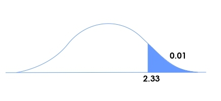
Step 4: Compute critical value. Since this test follows a t distribution, we are going to use t-table

Figure 1
Df = Smaller of n1-1 or n2-1 = 99
Looking into the t-table and locating 99 degrees of freedom, we got to know that Critical value is 2.33
Step 5: Reject speculation H0, there may be sufficient evidence to suggest that the students reading in increased software at a local excessive school have better rankings in mathematics issues than their comrades in Traditional layout programs.
Figure 2
Above mentioned formula is used in testing the difference of two population proportions using an independent sample. The test statistic has the usual everyday distribution. Each sample has to be large and each of the intervals has to lie inside [0, 1]. Let's look at the following example to perform the check
A permit to work on a residential project is issued to general contractors by the department of code enforcement of a county government. The result is inspected by the department which allows "pass" or "fail" certification, for each permit issued. Re-inspection of the failed permit maintains until it gets a bypass certificate. Since the department got frustrated by the high cost of re-inspection, it decided to publish the inspection record of all contractors on the web. It turned into the hope that public get entry to the statistics would lower the re-inspection fee. A year after the web access was made public, two samples of information were randomly decided on. One pattern became determined from the pool of records earlier than the netbook and one after. The proportion of initiatives that handed on the primary inspection turned into states for each sample. The outcomes are summarized under.
Construct a point estimate and a 90% self-belief c program language period for the difference in the passing fee on the first inspection among the 2 time periods. Now, test whether there is adequate proof to infer that open web access to the review records has expanded the proportion of ventures that passed on the principal assessment by over 5% points. Consider the critical value methodology at the 10% level of significance.
Read: An Easy Way to Understand Adaboost
Solution:
Step 1: Considering the naming of the populations an expansion in the passing rate at the main investigation by more than 5 % points after community on the web might be told as p1 <p2- 0.05, which through algebra is equivalent to p1 − p2 < − 0.05. Since the null hypothesis is continuously communicated as a correspondence, with the equal quantity at the privilege as is in the alternative speculation, the test is
H0 : p1 − p2 = − 0.05 vs. Ha : p1 − p2 < − 0.05 @ α = 0.10
Step 2: Since the test is as for a distinction in populations proportions the test measurement is given in Figure 3
Figure 3
Step 3: Inserting the values given in example and the value D0 = − 0.05 into the method for the check statistic gives value in the following given Figure 4
Figure 4
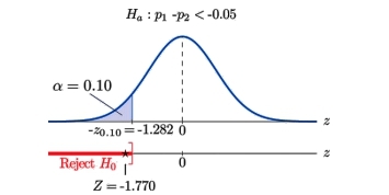
Step 4: Since the symbol in Ha is “<” this is a left-tailed test, so there is a single critical value, zα = − z0.10. From the last row in Figure 7.1.6 z0.10 = 1.282, so −z0.10 = − 1.282. The rejection region is (− ∞, − 1.282].
Step 5: As shown in Figure 5 the check statistic falls in the rejection region. The selection is to reject H0. In the context of the hassle our conclusion is:
The facts provide enough proof, at the 10% stage of significance, to conclude that the rate of passing on the primary inspection has accelerated through extra than 5 percentage points because records have been publicly published at the web.

Figure 5
A point estimate for the difference in population means is honestly the distinction within the corresponding sample method. In the context of estimating or trying out hypotheses concerning population means, "huge" samples approach that each sample is massive. A self-assurance c programming language for the difference in population means is computed the usage of a formulation inside the same style as became accomplished for a single population suggest. The most effective difference is in the method for the standardized take a look at the statistic.
When the statistics are collected in pairs, the variations computed for every pair are the data which are used within the formulation.
The identical five-step method used to check hypotheses concerning an unmarried population proportion is used to test hypotheses concerning the difference among population proportions. The simplest difference is within the formula for the standardized test statistic.
Please leave the query and comments in the comment section.
Read: 100+ Data Science Interview Questions and Answers
 Pinterest
 Email
Email
The JanBask Training Team includes certified professionals and expert writers dedicated to helping learners navigate their career journeys in QA, Cybersecurity, Salesforce, and more. Each article is carefully researched and reviewed to ensure quality and relevance.

Cyber Security

QA

Salesforce

Business Analyst

MS SQL Server

Data Science

DevOps

Hadoop

Python

Artificial Intelligence

Machine Learning

Tableau
Search Posts
Related Posts
A Complete Guide for Processing of Data
![]() 8.1k
8.1k
The Future of Data Science: Opportunities and Trends to Watch
![]() 4.8k
4.8k
Data Science Career Path: Your Roadmap to Become Data Scientist Pro
![]() 220.4k
220.4k
Prerequisite for Data Scientist: First Step To Becoming Data Scientist
![]() 5.6k
5.6k
List of Top 20 Data Science Tools For Visualization, Analysis
![]() 568.9k
568.9k
Receive Latest Materials and Offers on Data Science Course
Interviews