How to Do Data Manipulation of Packages Using R?

Introduction Data Manipulation

Data exploring is another terminology for data manipulation. It is simples taking the data and exploring within if the data is making any sense. Also, correcting the unwanted data sets. This will be done to enhance the accuracy of the data model, which might get build over time.

The data collection is one of the major key aspects. We will need to collect all the labelled data and unlabelled data from which ever sources required for the machine or the model to predict a good model.

Data treatment process/methods:

First and foremost, the method is to choose the right language to make the data. There are various languages R, Python, Java, Oracle, but the best is to find based on the data requirement. Each project has got its own base of treatment and process development.

Cream the R package gives a lot of quotes which helps to build or treatment process for the project. Similarly, there are various packages in python, which helps reduce the work activity. Help us to make the work very fast even optimising the code, move into production, testing, the data retreatment, and many other activities.

Machine learning this is very important for the data manipulation and to build a boosting algorithm to take care of the missing data, even its outliers and to find the corrupted parts of the data. If this is done manually, it is time-consuming and very less exercise. does be required a sophisticated tool to solve all these problems.

Packages used in R:

Here are some common add demonstrations for the use of packages in R.R

A). Dplyr

Created by Hadley Wickham. This package is very important for a programmer as it gives the basic features of filtering the data, select the data, manipulating it, and arranging it as per the business requirement. Also, it helps to summarise the data to present into the business world.

• filter – It filters the data based on a condition
• select – It is used to select columns of interest from a data set
• arrange – ascending or descending order arrangement of data
• mutate – It is used to create new variables from existing variables
• summarise (with group_by) – It is used to perform analysis by commonly used operations such as min, max, mean count, etc

B). SQL Queries or dplyr

Data is mostly stored in RDBMS format, and it is essential that people get used to it. How we can do in a scripting language. Many know queries that are written into a SQL language but needs to be converted into R function or a python function is a challenge. For which we can use similar ways like in SQL we have got select over here also they will be a function called select there is another condition based. So, the process remains almost similar. Below are the examples.

DPLYR Function	Equivalent SQL	Description
Select()	SELECT	Selecting Columns (variables)
Filter()	WHERE	Filter (Subset) rows.
Group_by ()	GROUP BY	Group the data
Summarise()	-	Summarise (or aggregate) data
Arrange()	ORDER BY	Sort the data
Join ()	JOIN	Joining data frames (tables)
Mutate ()	COLUMN ALIAS	Creating new Variables

Code Execution 'dplyr'

> if (!require('dplyr')) install.packages('dplyr',dependencies = T); library('dplyr')
> 
> # data()
> ########################### dplyr
> 
> data('iris')
> # Assigning the data
> mydata <- iris > # To view the data
> View(mydata)
> #To create local fram of the data and Viewing the data in the local data frame
> datairis <- tbl_df(mydata) > head(datairis)
# A tibble: 6 x 5
  Sepal.Length Sepal.Width Petal.Length Petal.Width Species
                                  
1          5.1         3.5          1.4         0.2 setosa 
2          4.9         3            1.4         0.2 setosa 
3          4.7         3.2          1.3         0.2 setosa 
4          4.6         3.1          1.5         0.2 setosa 
5          5           3.6          1.4         0.2 setosa 
6          5.4         3.9          1.7         0.4 setosa 
> 
> #Filtering the data based
> filter(datairis,  Sepal.Length > 1 & Sepal.Length < 54 )
# A tibble: 150 x 5
   Sepal.Length Sepal.Width Petal.Length Petal.Width Species
                                   
 1          5.1         3.5          1.4         0.2 setosa 
 2          4.9         3            1.4         0.2 setosa 
 3          4.7         3.2          1.3         0.2 setosa 
 4          4.6         3.1          1.5         0.2 setosa 
 5          5           3.6          1.4         0.2 setosa 
 6          5.4         3.9          1.7         0.4 setosa 
 7          4.6         3.4          1.4         0.3 setosa 
 8          5           3.4          1.5         0.2 setosa 
 9          4.4         2.9          1.4         0.2 setosa 
10          4.9         3.1          1.5         0.1 setosa 
# ... with 140 more rows
> table(datairis$Species)

    setosa versicolor  virginica 
        50         50         50 
> filter(datairis, Species %in% c('versicolor'))
# A tibble: 50 x 5
   Sepal.Length Sepal.Width Petal.Length Petal.Width Species   
                                      
 1          7           3.2          4.7         1.4 versicolor
 2          6.4         3.2          4.5         1.5 versicolor
 3          6.9         3.1          4.9         1.5 versicolor
 4          5.5         2.3          4           1.3 versicolor
 5          6.5         2.8          4.6         1.5 versicolor
 6          5.7         2.8          4.5         1.3 versicolor
 7          6.3         3.3          4.7         1.6 versicolor
 8          4.9         2.4          3.3         1   versicolor
 9          6.6         2.9          4.6         1.3 versicolor
10          5.2         2.7          3.9         1.4 versicolor
# ... with 40 more rows
> 
> #Selecting the column
> select(datairis, Sepal.Width)
# A tibble: 150 x 1
   Sepal.Width
         
 1         3.5
 2         3  
 3         3.2
 4         3.1
 5         3.6
 6         3.9
 7         3.4
 8         3.4
 9         2.9
10         3.1
# ... with 140 more rows
> #Removing the column
> select(datairis, -Petal.Length, -Species ) 
# A tibble: 150 x 3
   Sepal.Length Sepal.Width Petal.Width
                        
 1          5.1         3.5         0.2
 2          4.9         3           0.2
 3          4.7         3.2         0.2
 4          4.6         3.1         0.2
 5          5           3.6         0.2
 6          5.4         3.9         0.4
 7          4.6         3.4         0.3
 8          5           3.4         0.2
 9          4.4         2.9         0.2
10          4.9         3.1         0.1
# ... with 140 more rows
> select(datairis, -c(Petal.Length, Species))
# A tibble: 150 x 3
   Sepal.Length Sepal.Width Petal.Width
                        
 1          5.1         3.5         0.2
 2          4.9         3           0.2
 3          4.7         3.2         0.2
 4          4.6         3.1         0.2
 5          5           3.6         0.2
 6          5.4         3.9         0.4
 7          4.6         3.4         0.3
 8          5           3.4         0.2
 9          4.4         2.9         0.2
10          4.9         3.1         0.1
# ... with 140 more rows
> #select series of columns
> select(datairis, Sepal.Width:Species)
# A tibble: 150 x 4
   Sepal.Width Petal.Length Petal.Width Species
                           
 1         3.5          1.4         0.2 setosa 
 2         3            1.4         0.2 setosa 
 3         3.2          1.3         0.2 setosa 
 4         3.1          1.5         0.2 setosa 
 5         3.6          1.4         0.2 setosa 
 6         3.9          1.7         0.4 setosa 
 7         3.4          1.4         0.3 setosa 
 8         3.4          1.5         0.2 setosa 
 9         2.9          1.4         0.2 setosa 
10         3.1          1.5         0.1 setosa 
# ... with 140 more rows
> 
> #chaining
> datairis %>%
+   select(Sepal.Length, Petal.Length)%>%
+   filter(Petal.Length > 0.5)
# A tibble: 150 x 2
   Sepal.Length Petal.Length
                  
 1          5.1          1.4
 2          4.9          1.4
 3          4.7          1.3
 4          4.6          1.5
 5          5            1.4
 6          5.4          1.7
 7          4.6          1.4
 8          5            1.5
 9          4.4          1.4
10          4.9          1.5
# ... with 140 more rows
> 
> #arranging
> datairis %>%
+   select(Sepal.Length, Petal.Length)%>%
+   arrange(Petal.Length)
# A tibble: 150 x 2
   Sepal.Length Petal.Length
                  
 1          4.6          1  
 2          4.3          1.1
 3          5.8          1.2
 4          5            1.2
 5          4.7          1.3
 6          5.4          1.3
 7          5.5          1.3
 8          4.4          1.3
 9          5            1.3
10          4.5          1.3
# ... with 140 more rows
> 
> #or we can use
> datairis %>%
+   select(Sepal.Length, Petal.Length)%>%
+   arrange(desc(Petal.Length))
# A tibble: 150 x 2
   Sepal.Length Petal.Length
                  
 1          7.7          6.9
 2          7.7          6.7
 3          7.7          6.7
 4          7.6          6.6
 5          7.9          6.4
 6          7.3          6.3
 7          7.2          6.1
 8          7.4          6.1
 9          7.7          6.1
10          6.3          6  
# ... with 140 more rows
> 
> #mutating
> datairis %>%
+   select(Sepal.Length, Petal.Length)%>%
+   mutate(sepal.area = Sepal.Length * 12)
# A tibble: 150 x 3
   Sepal.Length Petal.Length sepal.area
                        
 1          5.1          1.4       61.2
 2          4.9          1.4       58.8
 3          4.7          1.3       56.4
 4          4.6          1.5       55.2
 5          5            1.4       60  
 6          5.4          1.7       64.8
 7          4.6          1.4       55.2
 8          5            1.5       60  
 9          4.4          1.4       52.8
10          4.9          1.5       58.8
# ... with 140 more rows
> 
> #summarising
> datairis %>%
+   group_by(Species)%>%
+   summarise(avg.Sepal.Length = mean(Sepal.Length))
# A tibble: 3 x 2
  Species    avg.Sepal.Length
                   
1 setosa                 5.01
2 versicolor             5.94
3 virginica              6.59
> 

C). data.table

This package allows you to manipulate the data at a faster level. Earlier they were many other traditional ways to perform the RDBMS data query sorry but now since the query languages sequel languages have changed, so the scripting has come, and we can get easily for late by using datatables. This requires minimum coding and maximum intellectual work focusing on the business.

Read: How Effective is the Graphics in R?

> ########################### data.table
> data("airquality")
> airqualitydata <- airquality > head(airquality)
  Ozone Solar.R Wind Temp Month Day
1    41     190  7.4   67     5   1
2    36     118  8.0   72     5   2
3    12     149 12.6   74     5   3
4    18     313 11.5   62     5   4
5    NA      NA 14.3   56     5   5
6    28      NA 14.9   66     5   6
> 
> #data table loading package
> library(data.table)
> airqualitydata <- data.table(airqualitydata) > airqualitydata
     Ozone Solar.R Wind Temp Month Day
  1:    41     190  7.4   67     5   1
  2:    36     118  8.0   72     5   2
  3:    12     149 12.6   74     5   3
  4:    18     313 11.5   62     5   4
  5:    NA      NA 14.3   56     5   5
 ---                                  
149:    30     193  6.9   70     9  26
150:    NA     145 13.2   77     9  27
151:    14     191 14.3   75     9  28
152:    18     131  8.0   76     9  29
153:    20     223 11.5   68     9  30
> 
> #selecting column
> airqualitydata[Ozone == 12]
   Ozone Solar.R Wind Temp Month Day
1:    12     149 12.6   74     5   3
2:    12     120 11.5   73     6  19
> 
> #selecting rows
> airqualitydata[1:3,]
   Ozone Solar.R Wind Temp Month Day
1:    41     190  7.4   67     5   1
2:    36     118  8.0   72     5   2
3:    12     149 12.6   74     5   3
> 
> #select columns with multiple values. This will give you columns with Setosa and virginica species
> table(airqualitydata$Day)

 1  2  3  4  5  6  7  8  9 10 11 12 13 14 15 16 17 18 19 20 21 22 23 24 25 26 27 28 29 30 31 
 5  5  5  5  5  5  5  5  5  5  5  5  5  5  5  5  5  5  5  5  5  5  5  5  5  5  5  5  5  5  3 
> airqualitydata[Day %in% c(3, 72)]
   Ozone Solar.R Wind Temp Month Day
1:    12     149 12.6   74     5   3
2:    NA     242 16.1   67     6   3
3:    32     236  9.2   81     7   3
4:    16      77  7.4   82     8   3
5:    73     183  2.8   93     9   3
> 
> #select columns
> airqualitydata[,sum(Ozone, na.rm = TRUE)]
[1] 4887
> airqualitydata[,Temp]
  [1] 67 72 74 62 56 66 65 59 61 69 74 69 66 68 58 64 66 57 68 62 59 73 61 61 57 58 57 67 81 79 76 78 74 67 84 85 79 82 87 90 87 93 92 82 80 79 77 72 65 73
 [51] 76 77 76 76 76 75 78 73 80 77 83 84 85 81 84 83 83 88 92 92 89 82 73 81 91 80 81 82 84 87 85 74 81 82 86 85 82 86 88 86 83 81 81 81 82 86 85 87 89 90
[101] 90 92 86 86 82 80 79 77 79 76 78 78 77 72 75 79 81 86 88 97 94 96 94 91 92 93 93 87 84 80 78 75 73 81 76 77 71 71 78 67 76 68 82 64 71 81 69 63 70 77
[151] 75 76 68
> airqualitydata[,.(Temp,Month)]
     Temp Month
  1:   67     5
  2:   72     5
  3:   74     5
  4:   62     5
  5:   56     5
 ---           
149:   70     9
150:   77     9
151:   75     9
152:   76     9
153:   68     9
> 

C). ggplot2

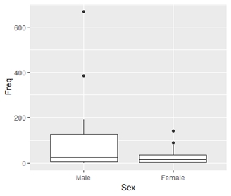
Making clothes are now much more is easier. Whatever baby required how much ever data we required; it is easy to formulate the graphs. Here are the three ways where we can use the GG plots to make the graphs:

• Scatter Plot
• Bar Plot
• Histogram

> ########################### ggplot2
> if (!require('ggplot2')) install.packages('ggplot2',dependencies = T); library('ggplot2')
> if (!require('gridExtra')) install.packages('gridExtra',dependencies = T); library('gridExtra')
> data('Titanic')
> TitanicData <- as.data.frame(Titanic) > class(TitanicData)
[1] "data.frame"
> 
> #boxplot
> colnames(TitanicData)
[1] "Class"    "Sex"      "Age"      "Survived" "Freq"    
> ggplot(TitanicData, aes(x = Sex, y = Freq)) + geom_boxplot() + theme(legend.position = 'none')

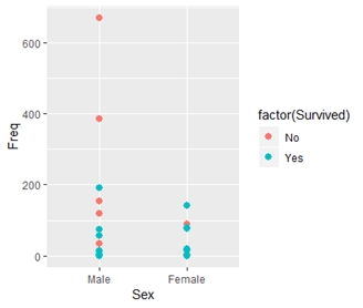
#scatterplot
> ggplot(TitanicData, aes(x = Sex, y = Freq, color = factor(Survived)))+geom_point(size = 2.5)

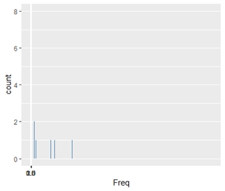
> #histogram
> ggplot(TitanicData, aes(x = Freq)) + geom_histogram(binwidth = 0.25, fill = 'steelblue')+scale_x_continuous(breaks=seq(0,3, by=0.5))

D). reshape2

Reshape is another important package which allows formulating the data into different forms. It allows us to aggregate and summarise data from large business set to a minimum required business set. Aggregation may use apply. This will help come over the problem we will be combined in many features to make the functions work.

Melt and cast are very important functions in this.

> ########################### reshape2 
> #Making New Data 
> id <- c(100,101,102,103,104,105) > name <- c('Ram','Lakhan','Rajesh','Pratham','Bharti','Guddi') > dob <- c(1988,1990,1975,1994,1992, 1995) > class1 <- c('Class1','Class1','Class1','Class2','Class2','Class2') > 
> datatem <- data.frame(id, name, dob, class1) > data.table(datatem)
    id    name  dob class1
1: 100     Ram 1988 Class1
2: 101  Lakhan 1990 Class1
3: 102  Rajesh 1975 Class1
4: 103 Pratham 1994 Class2
5: 104  Bharti 1992 Class2
6: 105   Guddi 1995 Class2
> 
> #load package
> if (!require('reshape2')) install.packages('reshape2',dependencies = T); library('reshape2')
Loading required package: reshape2

Attaching package: ‘reshape2’

The following object is masked from ‘package:tidyr’:

    smiths

The following objects are masked from ‘package:data.table’:

    dcast, melt

> #melt 
> melt(datatem, id=(c('id','name')))
    id    name variable  value
1  100     Ram      dob   1988
2  101  Lakhan      dob   1990
3  102  Rajesh      dob   1975
4  103 Pratham      dob   1994
5  104  Bharti      dob   1992
6  105   Guddi      dob   1995
7  100     Ram   class1 Class1
8  101  Lakhan   class1 Class1
9  102  Rajesh   class1 Class1
10 103 Pratham   class1 Class2
11 104  Bharti   class1 Class2
12 105   Guddi   class1 Class2
Warning message:
attributes are not identical across measure variables; they will be dropped 
> #cast
> dcast(melt(datatem, id=(c('id','name'))), dob + class1 ~ variable)
   dob class1  dob class1
1 1975 Class1 1975 Class1
2 1988 Class1 1988 Class1
3 1990 Class1 1990 Class1
4 1992 Class2 1992 Class2
5 1994 Class2 1994 Class2
6 1995 Class2 1995 Class2
Warning message:
attributes are not identical across measure variables; they will be dropped 
> 

E). reader

Read R is the parent directory for reading various files. The files can be its different forms of csv table xls etc. we need to be sure of which functions are we about to use for reading the data. There is another major factor that allows us while reading if you want the file to be in the same format as it is that is an example if a date formats to be selected then a date is selected if a character has to be selected for character selected.

factors(so no more stringAsFactors = FALSE
> ########################### readr  
> if (!require('readr')) install.packages('readr',dependencies = T); library('readr')
Loading required package: readr
> setwd("D:\\Janbask\\Personal\\JanBask\\data manipulation with r")
> # write.csv(datatem, "datatem.csv", row.names = FALSE)
> read.csv('datatem.csv')
   id    name  dob class1
1 100     Ram 1988 Class1
2 101  Lakhan 1990 Class1
3 102  Rajesh 1975 Class1
4 103 Pratham 1994 Class2
5 104  Bharti 1992 Class2
6 105   Guddi 1995 Class2
> 
> ########################### tidyr   
> if (!require('tidyr')) install.packages('tidyr',dependencies = T); library('tidyr')
> 
> # Adding the column
> timejoining <- c("27/01/2015 15:44","23/02/2015 23:24", "31/03/2015 19:15", "20/01/2015 20:52", "23/02/2015 07:46", "31/01/2015 01:55") > datatem_new <- data.frame(id, name, dob, class1, timejoining) > data.table(datatem_new)
    id    name  dob class1      timejoining
1: 100     Ram 1988 Class1 27/01/2015 15:44
2: 101  Lakhan 1990 Class1 23/02/2015 23:24
3: 102  Rajesh 1975 Class1 31/03/2015 19:15
4: 103 Pratham 1994 Class2 20/01/2015 20:52
5: 104  Bharti 1992 Class2 23/02/2015 07:46
6: 105   Guddi 1995 Class2 31/01/2015 01:55
> 
> #separating the date
> datatem_new %>% separate(timejoining, c('Date', 'Month','Year'))
   id    name  dob class1 Date Month Year
1 100     Ram 1988 Class1   27    01 2015
2 101  Lakhan 1990 Class1   23    02 2015
3 102  Rajesh 1975 Class1   31    03 2015
4 103 Pratham 1994 Class2   20    01 2015
5 104  Bharti 1992 Class2   23    02 2015
6 105   Guddi 1995 Class2   31    01 2015
Warning message:
Expected 3 pieces. Additional pieces discarded in 6 rows [1, 2, 3, 4, 5, 6]. 
> 
> #uniting the variables
> (datatem_new %>% separate(timejoining, c('Date', 'Month','Year'))) %>% unite(Time, c(Date, Month, Year), sep = "/")
   id    name  dob class1       Time
1 100     Ram 1988 Class1 27/01/2015
2 101  Lakhan 1990 Class1 23/02/2015
3 102  Rajesh 1975 Class1 31/03/2015
4 103 Pratham 1994 Class2 20/01/2015
5 104  Bharti 1992 Class2 23/02/2015
6 105   Guddi 1995 Class2 31/01/2015
Warning message:
Expected 3 pieces. Additional pieces discarded in 6 rows [1, 2, 3, 4, 5, 6]. 
> 

F). tidyr

This package allows us to tidy the data on the best of gathering spreading and separating as per the business requirement. Also, we can unite the data.

• gather() – it ‘gathers’ multiple columns. Then, it converts them into key: value pairs.
• spread() – It does reverse of gather.
• separate() – splits the column.
• unite() – It does reverse of separate. It unites multiple columns into a single column

G). lubridate

This package allowance to make the time variables more effective and easier to use and handle. All the time series plot in requires a lot of month on month data creation based on the time exact seconds etc.

Read: What Qualifications Are Required To Become Data Scientist?

> ########################### Lubridate 
> if (!require('lubridate')) install.packages('lubridate',dependencies = T); library('lubridate')
> 
> #check current time
> now()
[1] "2019-05-12 03:07:04 IST"
> 
> #assign to var
> var_time <- now() > var_time
[1] "2019-05-12 03:07:04 IST"
> var_update <- update(var_time, year = 2018, month = 11) > var_update
[1] "2018-11-12 03:07:04 IST"
> var_time_new <- now() > 
> # Checking the addition
> var_time_new + dhours(6)
[1] "2019-05-12 09:07:04 IST"
> var_time_new + dminutes(55)
[1] "2019-05-12 04:02:04 IST"
> var_time_new + dseconds(20)
[1] "2019-05-12 03:07:24 IST"
> var_time_new + ddays(3)
[1] "2019-05-15 03:07:04 IST"
> var_time_new + dweeks(4)
[1] "2019-06-09 03:07:04 IST"
> var_time_new + dyears(2)
[1] "2021-05-11 03:07:04 IST"
> 
> var_time$hour <- hour(now())
Warning message:
In var_time$hour <- hour(now()) : Coercing LHS to a list > var_time$minute <- minute(now()) > var_time$second <- second(now()) > var_time$month <- month(now()) > var_time$year <- year(now()) > 
> data.frame(var_time$hour, var_time$minute, var_time$second, var_time$month, var_time$year)
  var_time.hour var_time.minute var_time.second var_time.month var_time.year
1             3               7        4.850751              5          2019
> 

Apply () Function

To traverse the data, they are useless apply functions in various forms:

1). As Array/matrix

Apply function K versus S all the rows and columns of a matrix and apply the function to each of its resulting factors and return a result of summarised one.

2). List

The list is another important element, and it returns the result in an applied form sometimes it's also a possibility that simple resulting in a metric or vector. The result will be of the same length as it was in the starting, but the function annotation will be different.

apply(X, MARGIN, FUN, ...)

The apply() function takes four arguments as below:

X: This is the data—an array (or matrix)

> ########################### Apply() Function in R

> # Making matrix

> mat1<-matrix(c(seq(from=-88,to=1000,by=2)),nrow=5,ncol=5)

> # making product of each row

> apply(mat1,1,prod)

[1] -1299437568 -1111224576  -945229824  -799448832  -672000000

> # making sum of each row

> apply(mat1,2,sum)

[1] -420 -370 -320 -270 -220

Sapply () function

S apply does the same as the L apply, but in case it returns vector.

Tapply () function

Read: List of Top 20 Data Science Tools For Visualization, Analysis

T apply is used to calculate the mean median Max min or a simple function for each of the variables in a vector

Merge () Function

March is a very important function of R. In March by making the initial data set and the secondary data set based on a condition by which it is merging. If a left join must be performed, then we will be writing by.x followed by the column name. If the right join is to be performed then it will be by.y followed by the column name. We can also perform the full outer join full inner join and based on the business requirement. some of the examples are as below

> merge(data1, data2)

Here are the ways of doing the merge

Natural Join	Match each rose off the data sets whichever is on the merge	all=FALSE
Full Outer Join	to keep all the rows of both the data sets	all=TRUE
Left Outer Join in R	All the row of data set one taken as primary add merged	all.x=TRUE
Right Outer Join in R	All the rows of the data set two is taken as primary and merged	all.y=TRUE

Match () function

Match function returns the match in positions of the 2 data types or the vectors or more significantly vacancy positions of the very first matches that occur from one vector to another vector. Sir it is more like index match

> index <- match(data1$id, data2$id)

Conclusion

We have now seen how the data is manipulated and transformed as per the business requirement. Also, the joining of the data frames, apply function etc should be simple to understand. If you are keen in understanding and going deeper in R, then start working on simple problems by using the methods mentioned above.

Read: Logistic Regression is Easy to Understand

FaceBook Twitter Google+ LinkedIn Pinterest Email