02
JanChristmas Offer : Get Flat 50% OFF on Live Classes + $999 Worth of Study Material FREE! - SCHEDULE CALL
The Analysis of Variance (ANOVA) can be considered as a powerful applied mathematical tool for testing the significance. The test of significance supported t-distribution is an adequate procedure just for testing the importance of the distinction between two sample means. In a situation, once we have three or more samples to think about at a time an alternative procedure is required for testing the hypothesis that each one of the inputs is taken from the same population, i.e. they have the same mean.
Suppose, 5 different fertilizers are used in 4 plots each of which contains wheat and yield of wheat on each of the plots is given. We may be curious about checking whether the effect of those fertilizers on the yields is significantly different or in other words, whether the samples have come from the same normal population. The answer to the present problem is provided by the technique of analysis of variance. Thus, the basic purpose of the analysis of variance is to test the homogeneity of various means.
By ANOVA, the overall variation within the sample data is denoted as the sum of its non-negative components where each of these components is a measure of the variation due to some specific independent factors(causes) separately and then comparing these estimates due to assignable factors(causes) with the estimate due to chance factor(cause), the latter being known as experimental error or simply error.
The steps to design an experiment are:
Experiments have shown that proper consideration of the statistical analysis before the experiment is conducted, forces the experiments to plan more carefully the design of experiments. However, the certainty of the conclusion so drawn regarding the acceptance or rejection of the null hypothesis is given only in terms of probability. Accordingly, the design of the experiment may be defined as "the logical construction of the experiment in which the degree of uncertainty with which the inference is drawn may be well defined".
The basic principles of the design of an experiment are:

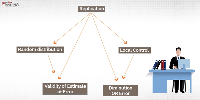
Replication can be explained as “the execution of an experiment more than once”. An experiment helps replication to average out the influence of the prospect factors on totally different experimental units. Thus, the repetition of treatment results in a more reliable estimate than is possible with a single observation. The following are the chief advantages of replication:
At the first instance, replication serves to reduce experimental error and thus enables us to obtain a more precise estimate of the treatment effects. From statistical theory, we already know that standard error (S.E.) of the mean of the sample of size n is σ / √n where σ is the standard deviation (per unit) of the population. Thus, if any treatment is repeated r times, then the S.E. of its mean impact is σ / √r, where σ2 is the variance of the individual plot is calculated from the error variance. Consequently, replication has an important but limited role in increasing the efficiency of the design.
The most important purpose of replication is to provide an estimate of the experimental error without which we cannot
As we already discussed, by replication the experimenter tries to average out as far as possible the effects due to uncontrolled effects. This brings to him the question of allocation of treatments to its worth. In the absence of the prior knowledge of the variability of the experimental material, this objective is achieved through “randomization”, a process of assigning the treatments to various experimental units in a purely chance manner. Randomization mainly focuses on:
The validity of the statistical tests of significance e.g. the t-test for testing the importance of the distinction between two means or the ‘Analysis of Variance’, F-test for testing the homogeneity of several means, based on the fact that the applied mathematics into consideration obeys some statistical distribution. Randomization provides a logical basis for that and makes it possible to draw rigorous inductive inferences by the use of statistical theories based on probability theory.
The purpose of randomness is to assure that the sources of variation, not controlled in the experiment, operate randomly so that the average effect on any group of units is zero.
It should be kept in mind that performing randomization only without performing replication is not enough. It is only when randomization of treatments to various units is accompanied by a sufficient number of replications then we are in a position to apply the test of significance.
If the experimental material, say field for agriculture experimentation, is heterogeneous and different treatments are allocated in various units(plots) at random over the entire field, the soil heterogeneity will also enter the uncontrolled factors and therefore increase the experimental error. It is mandatory to decrease the experimental error as much as possible without increasing the number of replications or without interfering with the statistical requirement of randomness so that the fewer differences between treatments can also be detected as important. The experimental error can be reduced by making use of the fact that neighbouring areas in a field are relatively more homogenous than those widely spread. To separate the soil fertility effects from the experimental error, the whole experimental area is divided into homogenous groups(blocks) row-wise or column-wise (one-way elimination of fertility gradient, c.f. Randomized Block design) or both (elimination of fertility gradient into two perpendicular directions c.f. Latin square design, according to the fertility gradient of the soil such that the variation within each block is minimum and between the blocks is maximum. The treatments are then assigned at random inside every block.
Read: How Effective is the Graphics in R?
The method of reducing the experimental error by dividing the comparatively heterogeneous experimental area(field) into homogenous blocks (due to physical closeness as for as field experiments are concerned) is known as Local control.
The Analysis of Variance (ANOVA) is mainly classified into two categories:
But here we are only discussing one-way classification.
Let us suppose that N observations xij (i=1,2,…..,k; j=1,2,…., ni ) of a random variable X are classified on some basis into k categories of sizes n1, n2,……., nk, (N=i=1kni ) as exhibited below:
| Means | Total | ||
| X11 | X12 …….x1n1 | x̄1 | T1 |
| X21 . . . . | X22 …….x2n2 . . . . . . . . | x̄2 . . . . | T2 . . . . |
| Xi1 | Xi2 …….xini | x̄i | T3 |
| Xk1 | Xk2 …….xknk | x̄k | T4 |
The total variation within the observation xij can be categorized into the following categories:
The first variety of a variable is because of negotiable causes which can be detected and managed by human endeavour and the second variety of variation is because of likelihood causes that are on the far side of the control of the human hand.
The main target of the ANOVA technique is to check whether there is enough difference between the class means because of the inherent variability inside the separate categories.
The linear mathematical model used in one-way classification is:
xij = µi + ij
= µ + (µi - µ) + £ij
= µ + i + £ij
where, (i=1,2,…..,k ; j=1,2,….,ni ),
xij is the yield from the jth cow, (j=1,2,…,ni) fed on the ith ration (i=1,2,…,k),
µ is general mean effect given by
µ=i=1kni µi / N,
Read: What do you Understand by AutoEncoders (AE)?
ai is the effect of the ith ration given by ai = µi - µ, (i=1,2,..k),
£ij is the error because of chance
Statistical analysis of the Model

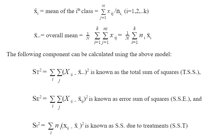
Hence,
Total S.S. = S.S.E + S.S.T
Degree of freedom for various S.S.
ST2, the total S.S. which is computed from N quantities of the form (xij - x̄..)2 will carry (N-1) degrees of freedom(d.f.).
Mean Sum of Squares (M.S.S.)
When we divide S.S by d.f then it gives M.S.S.
ANOVA Table for One-way Classification
|
Sources of Variation |
Sum of Squares |
d.f |
Mean Sum of Squares Read: An Easy To Interpret Method For Support Vector Machines |
|
Treatment (Ration) |
St2 |
k-1 |
st2= St2/(k-1) |
|
Error |
SE2 |
N-k |
SE2= SE2/(N-K) |
|
Total |
ST2 |
N-1 |
Conclusion
In this blog, we have discussed the Analysis of Variance (ANOVA). It is a statistical tool for the testing of significance. We have discussed the method for designing an experiment and also the classification of ANOVA. Further, One-way ANOVA is explained in detail, its approach, mathematical model, different sum of squares, degree of freedom and mean sum of squares.
Please leave the query and comments in the comment section.
Read: R Programming for Data Science: Tutorial Guide for beginners
 Pinterest
 Email
Email
The JanBask Training Team includes certified professionals and expert writers dedicated to helping learners navigate their career journeys in QA, Cybersecurity, Salesforce, and more. Each article is carefully researched and reviewed to ensure quality and relevance.

Cyber Security

QA

Salesforce

Business Analyst

MS SQL Server

Data Science

DevOps

Hadoop

Python

Artificial Intelligence

Machine Learning

Tableau
Search Posts
Related Posts
Random Forest: An Easy Explanation of the Forest
![]() 5.9k
5.9k
How to import Data into R using Excel, CSV, Text and XML
![]() 10.5k
10.5k
How Online Training is Better Than In-Person Training?
![]() 163.3k
163.3k
How To Write A Resume Of An Entry Level Data Scientist?
![]() 633k
633k
What Qualifications Are Required To Become Data Scientist?
![]() 808.5k
808.5k
Receive Latest Materials and Offers on Data Science Course
Interviews